What is Feature Engineering?
It can be difficult to find any sort of consensus on what the concept of “feature engineering” specifically refers to. Some people consider feature engineering to include data scrubbing steps that get your data into a format useable by machine learning (ML) algorithms. This includes steps such as dealing with missing values and outliers, encoding non-numerical data, and transforming and scaling variables. I tend to think of those things as steps in a preprocessing pipeline, separate from feature engineering. To me, feature engineering is mainly focused on using the variables you already have to create additional features that are (hopefully) better at representing the underlying structure of your data. But before we go any further, we need to step back and answer an important question.
What are Features?
A feature is not just any variable in a dataset. A feature is a variable that is important for predicting your specific target and addressing your specific question(s). For example, a variable that is fairly common to find across a diverse range of datasets is some form of unique identifier. This identifier may represent a unique individual, building, transaction, etc. Unique identifiers are very useful because they allow you to filter out duplicate entries or merge data tables, but unique IDs are not useful predictors. We wouldn’t include such a variable in our model because it would instantly overfit to the training data without providing any useful information for predicting future observations. Thus a unique ID is a variable, but not a feature.
So a feature can be thought of as a potentially useful predictor.
What is the Purpose of Feature Engineering?
Sometimes when you get your hands on a dataset, you might feel like you’ve got all the information necessary to tackle your problem. Usually this is not the case. So what can you do if you can’t go collect more data or measure additional variables? You can engineer features. Really what this means is applying domain knowledge to figure out how to use the information you do have in new and different ways to improve model performance. This is why it’s difficult to find resources covering the topic of feature engineering: it is so dependent on the domain you’re working within, your specific problem or task within that domain, the variables you already have, and the resources and ability you have to generate additional information.
Creating additional features that better emphasize the trends in your data has the potential to boost your model performance a great deal more than simply tuning hyperparameters. Just because the information is technically already there in your dataset does not mean a machine learning algorithm will be able to pick up on it. Important information can get lost amidst the noise and competing signals in a large feature space. Thus, in some ways, feature engineering is like trying to tell a model what aspects of the data are worth focusing on. This is where your domain knowledge and creativity as a data scientist can really shine!
When Should You Engineer Features?
As you explore the data you already have, here are a few questions to keep at the back of your mind:
- Is it possible to gain information or reduce noisy signals by representing the same variable in a different way?
- Do any of the variables have important threshold values that are not explicitly reflected in how the variables are represented?
- Can any of the variables be decomposed into two or more variables that would provide useful information?
- Can any of the variables be combined in some way to become more informative than the sum of their parts?
- Do you have information that would allow you to scrape or otherwise obtain useful external data?
If you answer “yes” to any of these questions, taking some time to engineer features is likely a useful endeavor.
Once you’ve engineered features, you’ll want to experiment with including and excluding different features when building your models. There are many approaches to feature selection, but those are outside the scope of this post. However, one thing to consider is that many of the features you engineer could be highly correlated with the variables you engineered them from. This may introduce issues with multicollinearity, especially if you’re working with linear models. On the other hand, tree-based algorithms may actually benefit from the inclusion of both the original and engineered features.
Examples of Feature Engineering
It’s really not possible to exhaustively cover all the possible ways of engineering features. However, below I’ve included a few instances of my own experience with attempting to engineer useful features. Even though these examples are very specific to a given problem, my hope is that my general thought process and snippets of code might prove useful to someone looking for inspiration for their own projects.
Example - Interaction Features: Sums
Let’s say you’re trying to predict whether someone gets the flu vaccine and you’ve got a dataset with information about the demographics, opinions, and relevant self-reported behavior of surveyed individuals. The behavioral variables are all binary, with a 1 representing that the individual engages in a behavior that decreases their risk of catching the flu, and 0 indicating that they don’t. If all the behavioral variables include the word ‘behavioral’ in the column name, you could pull out a list of all those variables with the following list comprehension:
behavior_cols = [col for col in flu_df.columns if 'behavioral' in col]
behavior_cols
[‘behavioral_avoidance’, ‘behavioral_face_mask’, ‘behavioral_wash_hands’, ‘behavioral_large_gatherings’, ‘behavioral_outside_home’, ‘behavioral_touch_face’]
There’s the list of all 6 behavioral variables. Each of these variables individually might be more or less useful for predicting flu vaccination status on its own, but we could also combine these variables to produce a metric indicating how much an individual adjusts their behavior to avoid contracting the flu. We could sum across each of these different behaviors to obtain such a behavioral score with the following code:
## use the behavior_cols defined above to specify columns to sum across
flu_df['behav_score'] = flu_df[behavior_cols].sum(axis=1)
Now we’ve got a variable ranging from 0 to 6, with higher values representing individuals that actively do more to avoid the flu.

Example - Indicator Variable/ Categories Based on Multiple Features
Based on domain knowledge, we know that certain individuals are at higher risk of developing flu-related complications. These individuals may be more motivated to get vaccinated, especially if they have multiple risk factors. We’ve got information on 3 major risk categories (whether they’re above the age of 65, whether they regularly come into contact with a young child, and whether they have a chronic medical condition), all represented by binary variables. The following block of code defines a function that scores an individual’s risk for developing complications, then applies it to create a new column:
## define a function to calculate score for high risk of complications
def calc_high_risk(row):
    risk = 0
    if row['older_65'] == 1:
        risk += 1
    if row['child_under_6_months'] == 1:
        risk += 1
    if row['chronic_med_condition'] == 1:
        risk += 1
    return risk

## apply the function to create new column
flu_df['high_risk'] = flu_df.apply(lambda x: calc_high_risk(x), axis=1)

## check the distribution of unique values in the new feature
flu_df['high_risk'].value_counts().to_frame()
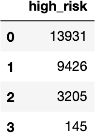
The function worked, but very few individuals have more than 2 risk factors. We could engineer a variable with less noise by grouping individuals with multiple risk factors (those with 2 or 3) with the following code:
## make a dictionary to map current values into risk categories
compl_map = {0:'low risk', 1:'med risk', 2:'high risk', 3:'high risk'}

## apply the map to the original column to create a new categorical variable
flu_df['high_risk_cat'] = flu_df['high_risk'].map(compl_map)

## check that the grouping worked
flu_df['high_risk_cat'].value_counts().to_frame()
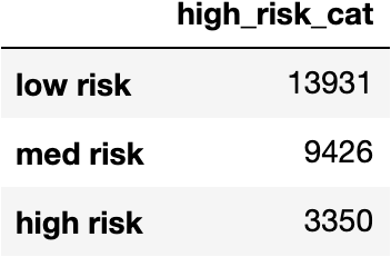
So now we’ve got individuals grouped into categories based on their heightened risk of developing dangerous complications. Binning or grouping rare categories can be a useful strategy when engineering more informative features to boost model performance.
Example - Decomposing Datetime Variables
If you ever work with a dataset that has dates and/or times, you’ll definitely want to make sure to do some feature engineering to decompose the original variables into useful features. Otherwise each date or timestamp will be treated as a relatively useless category. If you see you have some form of datetime information in your DataFrame, first check the data type. If it isn’t already in the form of a Pandas datetime variable, you’ll want to convert it to make use of some very useful methods for extracting information.
## use dtypes to check the type of data in our date column
house_df['date'].dtypes

## date is encoded as an object, so change it to a datetime variable
house_df['sold_dt'] = pd.to_datetime(house_df['date'])
Once we’ve cast the date as a datetime variable, we can easily extract date information in a form our model can learn from.
## import necessary library
import datetime as dt

## extract the month the house was sold
house_df['mo_sold'] = house_df['sold_dt'].dt.month

## extract the year the house was sold
house_df['yr_sold'] = house_df['sold_dt'].dt.year

## calculate the age of the house at the time it was sold based on the year it was built
house_df['age'] = house_df['sold_dt'].dt.year - house_df['yr_built']

## inspect new columns
house_df[['date', 'sold_dt', 'mo_sold', 'yr_sold', 'yr_built', 'age']].head()
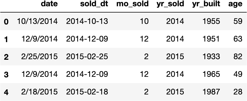
There are many ways to engineer useful features once you’ve got datetime variables. This sort of slicing works just as well when the variable includes time (hours, minutes, seconds) in addition to or instead of dates.
Example - Indicator Variable Using NumPy where()
This same house_df has information on the number of floors in each house. Some of the houses have half floors (a concept that confused and intrigued me since houses that have half floors probably have other similar elements to their design). However, as the floors variable currently stands, a model won’t necessarily pick up on houses that have half floors versus those that don’t. It will just focus on the total number of floors.
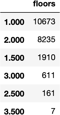
Additionally, it looks like we’ve got a rare label problem in that some categories are not especially common. This may introduce noise into the data that detracts from model performance. To highlight the distinction between houses with and without half floors for our model, we can create a new column with a binary indicator variable using NumPy’s where function:
## create a new column where a house gets a 1 if it has a half floor or a 0 if it doesn't
house_df['half_floor'] = np.where(house_df['floors'].isin([1.5, 2.5, 3.5]), 1, 0)


house_df[['floors', 'half_floor']][10:15]
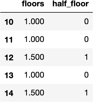
From here you might want to experiment with keeping the indicator variable and possibly rounding down the number of floors in the original floors variable. This would group the houses into fewer categories, getting rid of the rare labels.
In Conclusion
Feature engineering, like so many things in data science, is an iterative process. Investigating, experimenting, and doubling back to make adjustments are crucial. The insights you stand to gain into the structure of your data and the potential improvements to model performance are well worth the effort. Plus, if you’re relatively new to all this, feature engineering is a great way to get more comfortable working with and manipulating dataframes.